

Abstract
This project explores coding assistance as both a decision problem and a learning problem. On one side, I wanted to understand when an agent should surface a suggestion at all, since every intervention carries generation cost, verification cost, and the risk of distracting the user. On the other side, I wanted to build a system that could improve code generation itself through repeated execution, reward signals, and post-training.
That led to a two-part system. The first part is SimpleCoder, a ReAct-style CLI coding agent with bounded tool use, optional retrieval over the workspace, planning, context compaction, and permission-aware file access. The second part is a code RL post-training pipeline that samples code, executes it in a sandbox, converts outcomes into rewards, and updates the model through an iterative training loop. Together, they form a single idea: a useful coding agent should know when to help and should keep learning how to help better.
Introduction
Modern code assistants are often discussed as if generation quality were the whole story. But in practice, assistance quality depends on at least two separate questions.
The first question is intervention: when is it actually worth showing a suggestion? A suggestion may be correct and still be unhelpful if it costs more to inspect than it saves.
The second question is adaptation: once the model is producing code, how can its behavior be improved in a principled way rather than by prompt tweaking alone?
I treated this project as a bridge between those two questions. The modeling side gave me a framework for thinking about suggestion policies under uncertainty. The implementation side turned that framework into two working systems: one focused on inference-time interaction, and one focused on reward-driven improvement.
Modeling the Intervention Layer
Step 1: Modeling the Cost of Showing a Suggestion
The starting point is simple: showing a suggestion is not free. Even before a user decides whether to accept it, the system has already paid a generation latency cost and the user has already paid a verification cost.
If the suggestion is shown, the expected total time can be written as:
Here:
- is the time spent generating the suggestion
- is the time spent reading and checking it
- is the time needed if the user accepts but still edits
- is the time needed if the user rejects and writes manually
- is the probability that the suggestion is accepted
This equation matters because it shifts the problem away from raw model confidence and toward expected user effort.
Step 2: Turning Time into Utility
The next move is to compare this with the baseline of not showing anything at all. If the no-suggestion path costs , then the utility of showing becomes:
Substituting the previous expression gives:
This is the key simplification: once the time costs are fixed, the whole decision collapses onto the acceptance probability .
Step 3: Deriving the Threshold for Intervention
If writing from scratch is the default fallback, then . Under that assumption, showing is beneficial only when:
which gives the threshold:
That threshold is what I found most elegant in the model. It says the system does not need a vague sense that a suggestion is “probably useful.” It needs something sharper: the predicted acceptance rate must be high enough to overcome the combined burden of generation and inspection.
In other words, a coding assistant should intervene only when the expected savings justify the interruption.
Step 4: Why a Scalar Probability Is Enough
Another useful consequence of the model is that the raw context itself is not needed once it has been compressed into an estimate of acceptance.
Suppose the user state depends on context features and a candidate suggestion . The intervention decision can still be made entirely from the scalar prediction , because all of the contextual complexity has already been folded into that number.
That makes the control problem cleaner. The system does not need to reason over the full state every time it decides whether to show. It needs a reliable estimator of acceptance.
Step 5: Why Learning Is Necessary
Of course, the real acceptance probability is not directly observable. It depends on latent user state, which means the system has to learn an approximation such as:
or, more explicitly,
This is where the modeling in the PDFs becomes especially important. The decision rule is not useful by itself unless the estimated probability is reasonably calibrated. If is systematically too optimistic, the system will over-intervene. If it is too conservative, useful suggestions will be suppressed.
So the theoretical threshold only becomes operational once it is paired with a predictive model that can estimate acceptance from observable information.
Step 6: Uncertainty and the Two-Stage Policy
One of the nicest extensions in the modeling section is the move from a single-stage decision rule to a two-stage one.
If a lightweight context-only model already predicts with high certainty that a suggestion will be accepted or rejected, then it may be wasteful to generate a full suggestion just to confirm what is already obvious. But if the prediction is highly uncertain, then generation becomes worth paying for because it can change the decision.
That intuition can be described using entropy: when is near , uncertainty is high; when it is near or , uncertainty is low.
So the policy becomes:
- use a cheap context-only estimate when confidence is strong
- escalate to full suggestion generation only when uncertainty is high
This makes the system more computationally disciplined. It does not spend expensive generation effort on every interaction, only on ambiguous ones.
Step 7: Why Acceptance Rate Is a Bad Proxy
The final modeling insight I wanted to preserve from the PDFs is the critique of optimizing for acceptance alone.
If suggestion length is denoted by , an acceptance-oriented objective can be written as:
This type of objective can favor suggestions that are easy to accept because they are short and low-risk. But short, low-risk completions are not necessarily the ones that save the most time.
If the actual goal is time saved, the utility of an accepted suggestion is modeled as:
so the expected time saved becomes:
Since does not change the maximizer, the effective objective is:
If maximizes , then the condition for the time-optimal choice to move to the right is:
Equivalently,
or in ratio form,
That distinction captures a common failure mode in coding assistants. A system that optimizes for acceptance alone may learn to surface tiny, safe, nearly trivial completions. Those completions boost the metric, but they do not meaningfully improve productivity. The metric looks healthy while the user experience remains shallow.
For me, this was the conceptual center of the project: a good coding agent should optimize real utility, not just superficial agreement.
Modeling the Generator and Learning Signal
Step 8: Why One Reference Solution Is Not Enough
Once the suggestion policy is defined, the next question is where those suggestions come from. A natural baseline is supervised fine-tuning on reference solutions. If a model assigns probability to a solution for problem , then the standard SFT objective is:
In a finite dataset, that becomes:
For a sequence , the model factorizes autoregressively:
Therefore, the token-level negative log-likelihood expands as:
This is elegant, but it has a limitation that matters a lot for code. Many programming problems admit multiple correct implementations. If training pushes hard on only one reference trajectory, it can reduce probability mass on other valid solutions. In other words, SFT is faithful to the dataset, but not necessarily to the full solution set.
That is one of the reasons I found reward-based training more compelling for this project. Passing tests cares about semantic correctness, not stylistic imitation of a single reference answer.
Step 9: Binary Reward vs. Fractional Reward
Once code is executable, reward design becomes the next modeling choice. If a candidate passes tests out of , two obvious options are:
The fractional reward contains partial credit. It tells the model whether it is moving closer to a fully correct program even when it still fails some tests. That can make training denser and more informative.
At the same time, binary reward has a valuable strictness. It discourages opportunistic behavior that merely targets subsets of tests and instead forces the system to care about complete correctness. For code generation, that hard threshold often aligns better with how solutions are actually judged.
Step 10: What a Completion Pipeline Really Needs
Before any reward can be assigned, the system needs a concrete procedure for producing a candidate program. In practice, that means more than sampling tokens.
The generation pipeline has to:
- render the problem into the right prompt template
- tokenize and initialize the model state
- sample autoregressively under a decoding rule
- stop on conditions stronger than just max tokens
- decode the result into raw text
The stop conditions matter more than they first appear. End-of-sequence tokens, fenced code block termination, or explicit end markers all change the quality and cleanliness of outputs. If these controls are sloppy, evaluation becomes noisy before training even begins.
Step 11: Why Prompt Rendering and Extraction Are Part of the Environment
I ended up treating prompt rendering and code extraction as first-class parts of the system, not incidental preprocessing.
If a model is paired with the wrong chat template, several things can go wrong:
- role tokens may be interpreted as plain text
- system instructions may lose their priority
- the model may produce malformed or out-of-distribution outputs
Similarly, code extraction from raw model text has to be deterministic. If a response contains explanations and multiple code fences, the evaluator needs a rule for choosing exactly one program string or returning failure. This is not just cleanup. It directly affects reward.
That is why formatting became part of the environment design. A logically correct solution that is wrapped in unusable structure can still fail extraction and receive no useful reward.
Step 12: Why Safe Evaluation Requires a Sandbox
The moment code is executed in the loop, safety becomes non-negotiable. Running generated code through exec() on the host machine is not acceptable in any serious training pipeline.
There are at least two classes of failure:
- accidental failures, such as infinite loops, uncontrolled writes, or resource exhaustion
- adversarial failures, such as exfiltration of secrets, destructive shell commands, or malicious network behavior
This is why the sandbox is not auxiliary infrastructure. It is part of the learning environment itself. Without safe execution, automated code reward is not robust enough to trust.
Step 13: Reward Shaping and Its Tradeoffs
The shaped reward I used conceptually is:
and in the training setup this becomes:
with a small formatting coefficient.
I found the tradeoff here interesting. A negative formatting term helps the model distinguish malformed output from merely incorrect logic, which can accelerate learning of basic output discipline. But too much weight on format can also create a distorted incentive, where the model learns to produce safe-looking structure without solving the actual task well.
That tension is exactly the kind of thing I wanted this project to make visible: reward design is never neutral. It shapes what the model learns to care about.
Step 14: From Reward to Policy Gradient
Once a sampled completion receives a scalar reward , the objective is to maximize expected reward:
Writing the expectation explicitly:
Using the log-derivative trick, :
Switching back to expectation notation:
Since sequence probability factorizes over tokens,
so the final policy gradient becomes:
This is the bridge between automatic evaluation and learning. Once reward exists, token probabilities can be updated in the direction of solutions that perform better under execution.
Step 15: Baselines, Advantages, and Variance Reduction
Raw rewards are noisy, so the next refinement is to subtract a baseline and define:
The key reason this works is:
So subtracting the baseline leaves the expected gradient unchanged, while reducing variance. Intuitively, the model is no longer being told only “how good was this sample?” but rather “how good was this sample relative to what was expected for this problem?”
For grouped sampling, this becomes even cleaner. If we sample completions for the same prompt and define
then
because
This means the update is purely group-relative. The model is pushed toward completions that outperform their peers under the same prompt, and degenerate groups where all rewards are equal provide no learning signal at all.
That logic flows directly into GRPO. It is a neat fit for code generation because code rewards are sparse, high-variance, and naturally comparable within a prompt-conditioned group.
Code Deployment
Running SimpleCoder
The first implementation is packaged as a command-line tool. From the project root, the workflow is straightforward:
pip install -r requirements.txtpip install -e .simplecoder "create a hello.py file"simplecoder --use-rag "what does the Agent class do?"simplecoder --use-planning "create a web server with routes for home and about"simplecoder --interactiveThis deployment model keeps the agent lightweight. It behaves more like a controlled coding utility than a general-purpose assistant shell.
Running the RL Pipeline
The second implementation depends on sandboxed execution, so its setup is slightly more infrastructural. After installing requirements, I start the Sandbox Fusion server and then run train.py.
python -m pip install -r requirements.txtdocker run -it -p 8080:8080 -v ./sandbox_config/local.yaml:/root/sandbox/sandbox/configs/local.yaml volcengine/sandbox-fusion:server-20250609python train.pyThe same training script supports two backends:
backend=tinkerfor remote trainingbackend=local_gpufor local LoRA fine-tuning
That split made the project easier to iterate on, since the same overall training logic could be tested under different compute conditions.
Implementation
Part I: SimpleCoder
ReAct-Style Agent Loop
At its core, SimpleCoder uses a ReAct-style interaction loop. The model reasons about the task, invokes tools, observes the results, and continues until it can return an answer or produce an output. This makes the system better suited to coding work than a pure one-shot completion model, because many coding tasks require inspection before generation.
Bounded Tooling
The tool registry exposes a small set of actions:
read_filewrite_filelist_filessearch_in_files
I liked this design because it keeps the tool surface narrow and predictable. Reads and searches can inspect the workspace, while writes are constrained to a designated output root. That separation makes the agent useful without letting file mutation become arbitrary.
Retrieval Over Code
The RAG layer builds a temporary vector index by chunking files into line-based segments, embedding those segments, and retrieving the most relevant ones at query time. Instead of flooding the model with entire files, the system can pass only the pieces most likely to matter.
For code-heavy work, that matters a lot. It reduces context waste and improves grounding in larger repositories.
Planning and Context Compaction
The planner provides a coarse sequence of steps before execution. It is not meant to replace reasoning inside the loop, but it gives the run a more structured trajectory.
The context manager solves a different problem: long coding sessions can overwhelm the prompt window. Once the message history grows beyond a threshold, older turns are summarized and folded into a compact state representation. That keeps the conversation coherent without letting prompt length grow indefinitely.
Permission-Aware Interaction
One of the more practical features is the permissions layer. Reads and writes are guarded, and the user can approve actions once or persist the decision across runs.
This is a small detail, but it changes the feel of the agent. It turns file access into an explicit contract instead of an invisible capability.
Part II: Code RL Post-Training
Sandbox-Evaluated Code Generation
The training system treats code quality as something that must be tested, not merely judged by fluency. Candidate solutions are sampled and then executed inside a sandbox, where their behavior can be scored against task requirements.
That evaluation loop is what anchors the training signal to actual program behavior.
Rewards, Advantages, and Datums
The structure of the training loop is intentionally minimal and explicit. The main functions ask four questions:
- should this batch be skipped?
- what advantages should be computed from the observed rewards?
- how should a token trajectory be packaged into a training datum?
- how should the optimizer step be applied?
This decomposition keeps the RL logic readable. Rather than burying everything inside a single training script, the loop is expressed in stages: sampling, evaluation, reward attribution, and update.
Dual Training Backends
I implemented two training paths:
- a Tinker-based remote backend
- a local GPU backend with LoRA fine-tuning
This was useful both practically and conceptually. Practically, it meant I could run the same high-level experiment under different compute environments. Conceptually, it emphasized that the core contribution was not tied to one specific infrastructure choice. The important part was the reward-driven training loop around executable code.
Logging, Checkpoints, and Run Evidence
The system writes logs, metrics, checkpoints, and trend plots under timestamped run directories. That turns each run into a traceable artifact rather than a black-box training attempt.
I found this especially important for a project like this, because post-training claims are only convincing when the evidence remains inspectable after the run is over.
Results and Takeaways
The clearest signal came from the Tinker training run over 100 steps. The best correctness metric improved from 0.4043 to 0.5195, while reward improved from 0.3961 to 0.5164. Loss also dropped dramatically, with the strongest checkpoint appearing at step 56.
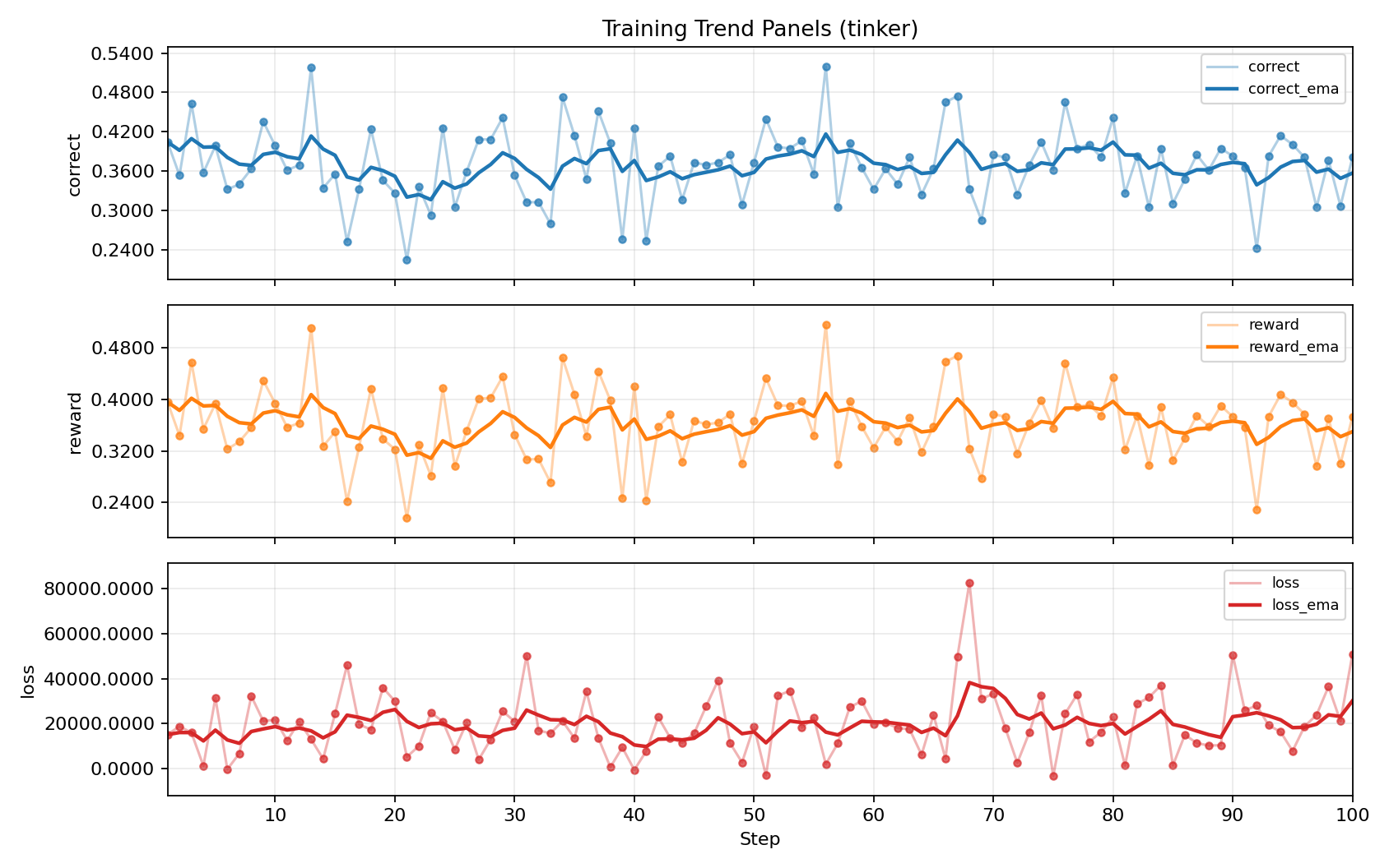
What I find most compelling is not just that the metrics moved, but why they moved. The system was not being rewarded for sounding plausible. It was being rewarded for generating code that survived execution-based evaluation. That gives the improvement a more meaningful interpretation.
More broadly, the project convinced me that coding agents should be designed as layered decision systems.
- A good assistant needs an intervention policy so it knows when speaking is worth the cost.
- It also needs a generation policy that can actually produce code worth accepting.
- And once those outputs are testable, it needs a feedback loop that turns behavior into learning.
If any one of those layers is weak, the overall experience degrades. A cautious but mediocre assistant becomes timid. A strong generator with no intervention discipline becomes noisy. A polished interface without a learning loop quickly plateaus.
Given the limited training budget, modest data scale, and high-variance nature of code RL, I did not expect the run to converge cleanly. The fluctuations in reward and correctness are noticeable, and the overall result is better understood as evidence that the pipeline is wired correctly and capable of improvement, rather than as a fully stabilized training outcome.
Closing Thoughts
What stayed with me after this project was how much of coding assistance is really about control, not just generation.
The modeling side forced me to think carefully about interruption, uncertainty, and user effort. The implementation side forced me to think about bounded action, retrieval, execution, and feedback. Put together, those pieces suggest a view of code agents that is more structured than autocomplete and more honest than raw demo metrics.
For me, that is the real value of this project. It is not just a coding assistant and not just a training pipeline. It is an attempt to connect theory, interface behavior, and post-training into one coherent system for adaptive help.